The following report intends to analyze avocado prices and sales volume from 2015 to early 2018 across the US. In addition to a thorough exploratory analysis, I’ll also try to calculate the price elasticity of demand for each individual market. The dataset comes from the Hass Avocado Board.
Data Pre-Processing
Load Data
#load avocado data
load("data/avocados.Rda")
Load Packages
library(tidyverse)
library(scales)
library(plotly)
library(wesanderson)
Clean Data
The dataset contains weekly average prices and total amount sold for both organic and conventional avocados for 45 different markets (New York, Boise, St. Louis, etc.) that make up 8 larger regions (California, Great Lakes, Midsouth, Northeast, Plains, South Central, Southeast, and West). I’ll create three different datasets: one containing the 45 markets, one for the 8 larger regions, and one for entire US. Also, three price lookup codes (PLU’s) are listed, but for Hass avocados only, so I’ll create another variable to hold the rest of avocados (e.g. green-skinned) sold per week.
#replace spaces with underscores in column names
names(avocados) <- gsub(" ", "_", names(avocados))

#rename PLU codes and tidy up data
avocados <- avocados %>%
  rename(small_hass = "4046", large_hass = "4225", xl_hass = "4770") %>%
  mutate(other = Total_Volume - small_hass - large_hass - xl_hass) %>%
  gather(bag_size, bag_total, c(Small_Bags, Large_Bags, XLarge_Bags)) %>%
  gather(avocado_type, avocado_volume, c(small_hass, large_hass, xl_hass,
                                         other))

#subset data by region
avocados_region <- avocados %>%
  filter(region %in% c("California", "West", "SouthCentral", "GreatLakes",
                       "Midsouth", "Southeast", "Northeast", "Plains"))

#subset data by market (city)
avocados_market <- avocados %>%
  filter(!(region %in% c("California", "West", "SouthCentral", "GreatLakes",
                       "Midsouth", "Southeast", "Northeast", "Plains",
                       "TotalUS")))

#dataset for entire US
avocados_total <- avocados %>%
  filter(region == "TotalUS")
Let’s make sure we don’t have any missing values
paste(sum(is.na(avocados_market)),
sum(is.na(avocados_region)),
sum(is.na(avocados_total)))
## [1] "0 0 0"Bravocado! Also, let’s see if there are any hidden markets that make up a region.
cat(paste("Market Volume:",
sum(avocados_market$avocado_volume),"\n"),
paste("Region Volume:",
sum(avocados_region$avocado_volume), "\n"),
paste("Total Volume:",
sum(avocados_total$avocado_volume)))
## Market Volume: 11381766688.74
## Region Volume: 17594220546.06
## Total Volume: 17594220545.4So it looks like some avocados (6,212,453,857 to be exact) were sold over the past few years in markets not found in the dataset. But the eight regions do in fact contain the entirety of US avocado sales (minus rounding error).
Exploratory Data Analysis
Distribution
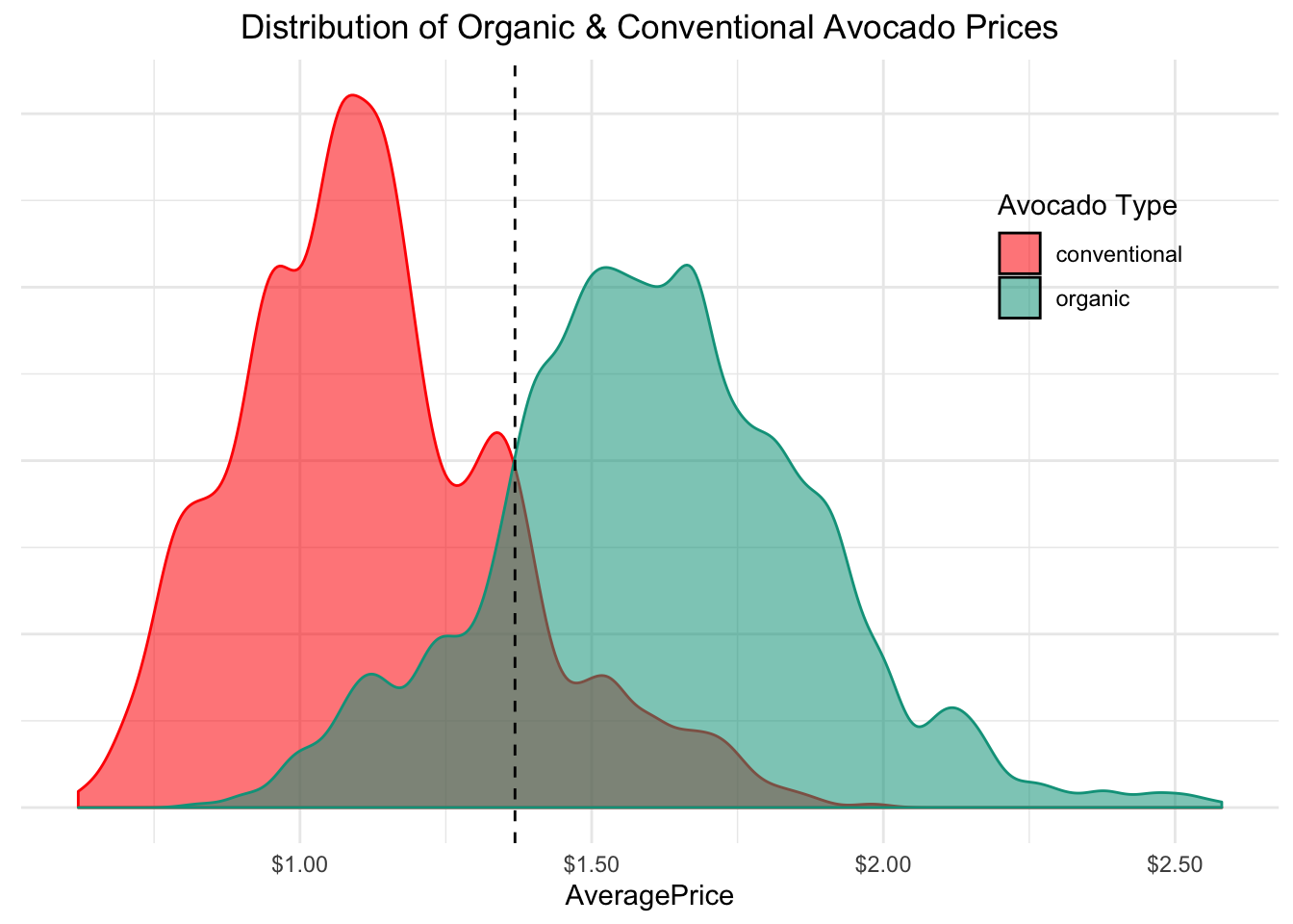
Alright now that we understand the data, I think it’s time for some exploratory data analysis! First, let’s look at how the prices of organic and conventional avocados are distributed.

Not surprisingly, organic avocados are generally priced higher than conventional ones. The dashed vertical line in the middle represents the average weekly price for all avocados, $1.37. Next, let’s look at how prices have varied over time.
Avocado Prices
A couple of things stick out to me. Avocados reached a 3-year high in late summer 2017. Also the apocalyptic organic price drop around July 2015. My guess is that there was some missing data for US total organic avocado prices in July 2015 that got imputed as $1.00. Let’s check the price movement for each region to see if any sharp declines in July 2015 exist.

Nothing out of the ordinary here. Organic prices never dropped below conventional prices in each region. I will just leave the US dataset as is and focus the rest of my analysis on the region dataset. Now, let’s see how avocado prices vary across regions.

The Northeast region sells avocados at the highest average price. Now, let’s determine which size of avocados each region buys.
Avocado Volume

The South Central, California, and West regions make up the three largest avocado regions by volume. The Northeast region sells the most Large Hass avocados (both proportionally to total regional sales and overall) which probably contributes to them having the highest average price. With that said, let’s look at how each market consumes avocados.

The LA market appears to be ripe for avocados; it doubles the second largest market (New York) in terms of volume. Avocados seem to be most popular in western or warm weathered markets. Even smaller markets like Denver and Portland rank near the top among the larger US cities suggesting avocado consumption has a geographical element to it.
Elasticity
Finally let’s look at the price elasticity of avocados. We can try to determine which markets avocados are the most price elastic. First, let’s plot total volume against average price for all avocados.

Conventional avocados appear to show a linear relationship. It’s hard to make up the shape for the organic avocados so let’s try plotting each type in its own graph. It’s also worth noting that organic avocados are sold in much lower volumes than conventional avocados.

It looks like the organic avocado price vs. sales relationship is more uniform, hinting that it has a less elastic demand than conventional avocados. The linear model seems to do an adequate job of describing the data so, for simplicity, let’s just fit a linear price-response function for all markets and compare their overall elasticities.
elas <- lapply(unique(avocados_market$region), function(b){
            df <- avocados_market %>%
              filter(region == b)
            m <- lm(Total_Volume ~ AveragePrice, data = df)
            x <- m$coefficients[["AveragePrice"]]
            y <- mean(df$AveragePrice)
            z <- mean(df$Total_Volume)
            x*y/z
        })

elas <- do.call(rbind, elas) %>%
  data.frame() %>%
  mutate(market = unique(avocados_market$region)) %>%
  mutate(elasticity = round(., 2)) %>%
  select(-c(.))
The overall demand for avocados is elastic in all markets. Western markets (especially the Pacific Northwest) are typically less responsive to changes in price than eastern markets. A 10% price increase would cause an 18% drop in demand in Seattle but a 37% drop in New York. The Pittsburgh market could very well be immune to the avocado craze as a 10% price increase would decrease demand by 58%, 20% more than the next closest market, fellow Pennsylvanian city, Philadelphia.